RebellionResearch.com White Paper - Volume 2.0
Data and Measurement
We begin by describing our KRX intra data of stocks hitting the upper price limit. We then describe our measure of the influence of a individual buyer.
2.1 Data
We use the intraday transaction data for stocks listed on the KRX from February 1, 2008
through December 30, 2009 (479 trading days). The transaction data include the price and quantity of stocks sold or bought, and the trade time in milliseconds. The symbol that uniquely identifies an account is given for each trade. Although the original data covers everyday trading for all stock on the KRX, we only use the data of stocks hitting the upper price limit as our sample.
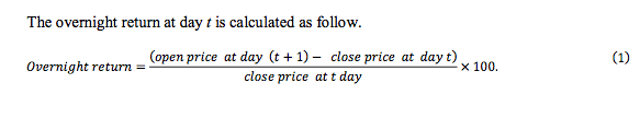
We impose two filters on our initial sample. First we require our data to include only firms that have a next day open price to estimate overnight return. Second we remove all observations with overnight returns larger than 15% to exclude recording errors in the sample. As a result, 7 observations were removed. These requirements leave 19,069 observations from 1,788 stocks.
Panel A of Table 1 presents the distribution of the number of stocks hitting the upper price limit in a day. It was on October 30, 2008 (the day with most hits) when 843 stocks hit the upper price limit. On that day, KOSPI index increases 11.95 percent point, which is the highest record ever in KRX and KOSDAQ index also increase 11.47 percent point.
Panel A of Table 1 shows that although approximately 40 stocks hit the upper price limit as close price in a day on average, standard deviation is around 46, which is larger than the mean. The reason we observe much larger standard deviation than its mean is that we have extreme outliers such as the day of October 30, 2008. Only with observations which have hit less than 100, the mean and the standard deviation are 35.056 and 18.081, respectively. Our main results are calculated from the full sample, and we include robustness tests with this sub-sample of hitting less than 100.
Panel B of Table 1 shows the distribution of hitting the upper price limit. Each stock hits the upper price limit approximately 10 times on average for a whole period. In particular, 2 Because of this requirement, we can’t use the sample data of last day(479th day). 61,121 firms hit the upper price limit less than 10 times, which account for 63.04% of all sample firms, 1,778.
Panel C of Table 1 shows the distribution of the duration of day for a stock hitting the upper price limit continuously. For example, if stock hits the upper price limit, in the next day the stock does not hit the upper price limit, and after several trading days, the stock again hits the upper price limit, then we consider the stock as two different samples in the distribution. From the distribution, we can estimate the probability of a firm hitting the upper price limit in the next day assuming that the firm hit the upper price limit today, which is 21.71%
Panel A of Table 2 shows the percentile and the summary statics of overnight return. If a stock hits the upper price limit, the stock shows around 4.6% of overnight return in the next day which is statistically different from 0 with the t-statistic of 122.72. Panel B of Table 2 shows the number of samples in three categories: sample with positive overnight return, sample with zero overnight return, and sample with negative overnight return. Among 19,069 observations, 14,865 show positive return, 1,426 show zero overnight return, and 2,778 show negative overnight return. Based upon these statistics, we can estimate the probability of a stock price rising the next day if the stock price hit the upper price limit today. As in the third column in Panel B of Table 2, the probability of a stock price rising the next day if the stock price hits the upper price limit today is 77.95%, which is
This is calculated by extracting the ratio of sample of first bin of the histogram, 78.29%, from 100%
approximately five times larger than the probability of a stock price decreasing the next day if the stock price hits the upper price limit today,14.57%.
2.2 Influence of a buyer(IB)
Although two different stocks A and B hit the upper price limit, the procedures hitting the upper price limit may be different. Among the various difference of the procedures, we focus on the number of investors.
In particular, we focus on the number of sellers traded with a buyer on average in a day for a stock, equivalently, the ratio of the total number of sellers relative to the total number of buyer in the day for the stock. We name the number or the ratio as ‘the influence of a buyer (IB)’.
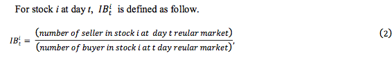
Where "number of sellers in stock i at a day t regular market" and "number of buyers in stock i at day t regular market" are calculated using the notion of ‘net’ buyer and ‘net’ seller. Suppose that an investor sells 𝑄1 amount of stock i and buys 𝑄2 amount of stock i at day t regular market. If Q1 < Q2, then the investor is only included in "number of buyers in stock i at day t regular market"
If IB i/t is lower than 1, there exist more buyers than sellers in stock i at day t, and vice versa. In general, if IB i/t is ‘p’, then it means that, on average, each buyer has traded stock i with ‘p’ sellers at day t, equivalently there is ‘p’ times more sellers than buyers. So, with larger IB i/t, there are more sellers with whom each buyer trades on average.
Table 3 shows the descriptive and the summary statics of the IB. The mean of IB is statistically different from 1 with the t-statistic of 29.79, but the median of IB is 1.06 with much smaller statistical significance (XXXX). This test means that the number of sellers are larger than the number of buyers when stock hits the upper price limit.
3. Result
3.1 IB and overnight return
To study the relationship between IB and overnight return, we analyze our sample in two
different ways: day-by-day grouping (Panel A) and whole sample period grouping (Panel B).
In the analysis of the day-by-day grouping, we sort 478 daily samples into deciles day by day so that we can get 478 bundles of 10 groups. Then, we aggregate each decile across time and calculate average overnight return and the difference of average overnight returns. By applying the day-by-day grouping, we can control the daily effect in the market. In the analysis of the whole sample period grouping, 10 groups are constructed based upon IB in the whole sample period without considering daily effects.
As in Panel A of table 1, there are two days (20091014 and 20091028) when the number of firms hitting the upper price limit in a day is smaller than 10. Therefore, we exclude the observations in these two days
from our sample to implement the day-by-day analysis. In total, 17 observations are excluded from our sample.
Panel A shows the results from the analysis using day-by-day grouping. It presents the average overnight return and difference of average overnight returns between each of 10 groups and the max or the min IB group. The average overnight return of group 1 (min IB) is 5.7%, which is the second largest. After the average overnight return drastically decreases in group 2, 3.97%, the average overnight returns are approximately similar in group 2-7, in the range of 3.80-4.11%. But going through from group 7 to group 10 (max IB group), average overnight returns increase significantly, from 4.11-6.56%. In short, group 1 (min IB) and group 10 (max IB), show the two largest overnight returns whereas with the middle groups, groups 2 - 9, the average overnight returns have relatively smaller value and show an upward trend.
Therefore, the overnight return has a U shape across 10 groups, and the standard errors of average return in 10 groups show that the U shape is economically and statistically significant at all conventional levels.
The differences of average overnight returns between group 10 (max IB) and each other group are positive and have a flipped U shape.
The t-statistics of two sample t-tests between group 10 (max IB) and the other groups are large enough to be statistically significant, ranging from 4.46 to 15.42. The differences of average overnight returns between group 1 (min IB) and each group are also mostly positive and also have a flipped U shape. Except for the case with group 10 (the t-statistic of -4.46), t-statistics of two sample t-tests between group 1 and other groups other than group 10 report statistical significance from 2.11 to 10.04. Therefore, the differences of the average overnight return also support the previous results that the overnight return has a U-shape across 10 groups and the shape of U is economically and statistically significant at all conventional levels.
As shown in panel B of table 4, similar results are obtained in the analysis using a whole
sample period. Group 1 (min IB) and group 10 (max IB) show the two largest average 10
overnight returns whereas the middle groups, groups 2 - 9, have relatively smaller values similar to the previous analysis with the day by day grouping. In summary, the average overnight return also takes a U-shape across 10 groups and this empirical observation is economically and statistically significant at all conventional levels.
3.2 Herding effect on each group
To measure herding effect of each group, we develop three herding measures based on the herding measure by Lakonishok, Shleifer and Vishny (1992).
To be continued in Volume 3.0
Edited by Alexander Fleiss
Read more from RebellionResearch.com:
Why a Machine Learning Investment?
Interview with Astronaut Scott Kelly: An American Hero
AQUAPONICS: How Advanced Technology Grows Vegetables In The Desert
A New Breed of Airline Looks to Take the World by Storm!
$91 Million for a Pair of Gloves: Chelsea Leads Global Sports' Spending Spree
The World Cup Does Not Have a Lasting Positive Impact on Hosting Countries…
Dating Wine Using Nuclear Signatures
Baseball Attendance Keeps Falling
Giancarlo Stanton: A $300 Million Dollar Question Mark
A Conversation with Boston Red Sox Vice President of Player Personnel
Derek Jeter is Facing up to Half a Billion Dollars of Losses on the Miami Marlins
On Black Holes: Gateway to Another Dimension, or Ghosts of Stars’ Pasts?
Are Derek Jeter & the Miami Marlins Going to Face a Cash Crunch?